Analysis Demo

# Disable warnings for prettier notebook
import warnings
warnings.filterwarnings("ignore")

from pathlib import Path
import matplotlib.pyplot as plt

import pandas as pd
import numpy as np

import torch

import anndata as ad
import scanpy as sc
import squidpy as sq

from popari import pl, tl
from popari.model import load_trained_model

Load trained model

data_directory = Path("/work/magroup/shahula/spatiotemporal_transcriptomics_integration/data/STARmapPlus/SCP1375/")
demo = load_trained_model(data_directory / f"hierarchical_results", verbose=0, context=dict(device="cuda:0", dtype=torch.float64)) # Replace with path to your trained model

Load from MLflow

from popari.mlflow.util import load_from_mlflow_run

If you used the MLflow to run a grid search for Popari hyperparameters, you can load your favorite run using the load_from_mlflow_run function.

Generic analyses

Most functions in the tl and pl libraries can accept a level argument, which specifies the level of the hierarchical representation that the function should be executed at. We begin by applying all functions at level=1 (the highest available level).

Postprocessing

First, we Z-score normalize the Popari embeddings; this ensures that the dimensions of the latent space are weighted equally for downstream tasks such as clustering.

tl.preprocess_embeddings(demo, level=1, normalized_key="normalized_X")

We can also compute the empirical correlation between the learned embeddings X, and these results can later be compared/contrasted against the learned spatial affinities.

tl.compute_empirical_correlations(demo, level=1, feature="X")

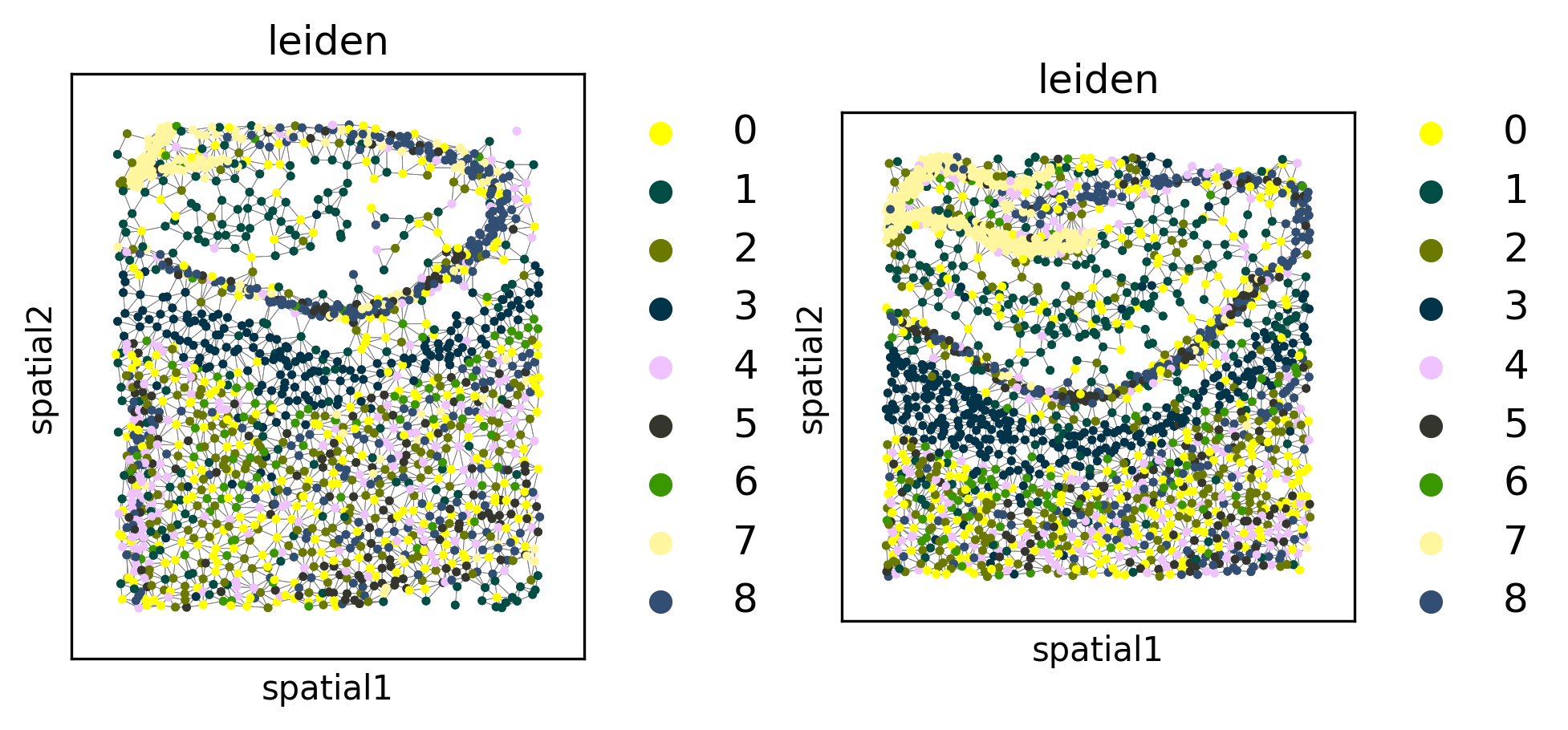
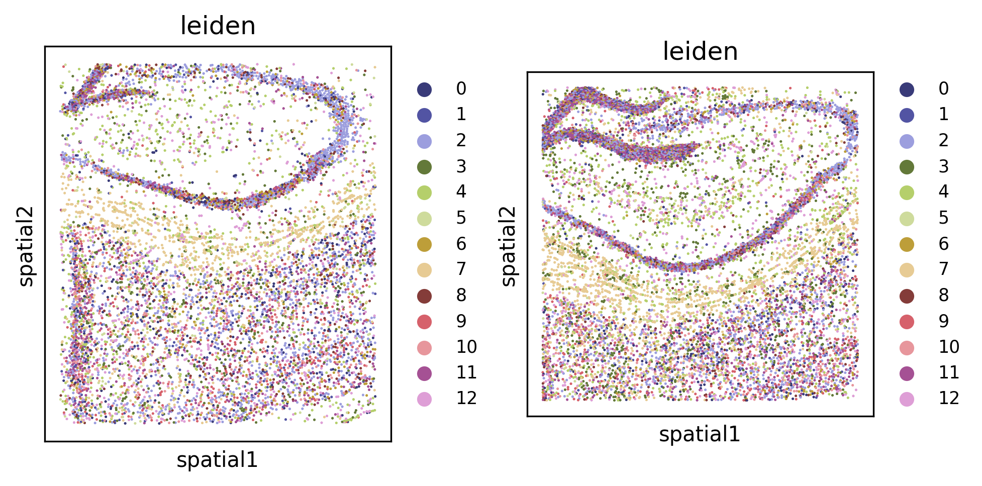
Leiden clustering

We can cluster the embeddings to uncover cell types or other spatially-coherent groupings of the samples. The clustering can either be done separately for each FOV (default), or jointly for all datasets (using joint=True).

tl.leiden(demo, level=1, joint=True, use_rep="normalized_X")

fig, axes = plt.subplots(1, 2, constrained_layout=True, dpi=300, squeeze=False)
_ = pl.in_situ(demo, color="leiden", level=1, size=10, legend_fontsize="large", joint=True, axes=axes)

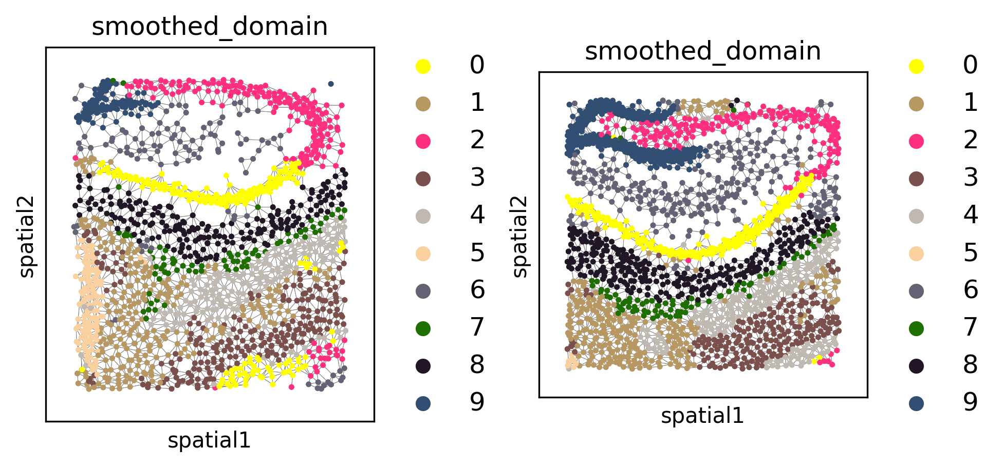
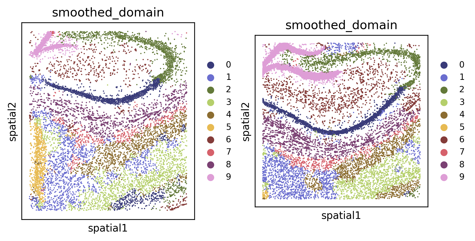
Spatial domain clustering

We can also cluster for spatial domains. This also employs Leiden clustering under the hood, but it includes several noise-reduction/spatial smoothing priors to improve the performance of spatial domain segmentation.

tl.cluster_domains(demo, level=1, target_domains=None) # writes inferred domains at key "smoothed_domain" for each f 

Processing datasets eight_month_level_1 <=> thirteen_month_level_1

fig, axes = plt.subplots(1, 2, constrained_layout=True, dpi=300, squeeze=False)
_ = pl.in_situ(demo, color="smoothed_domain", level=1, size=10, legend_fontsize="large", joint=True, axes=axes)

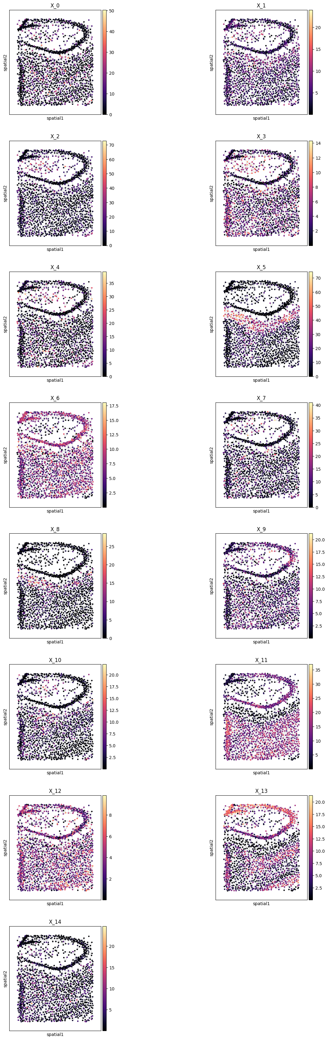
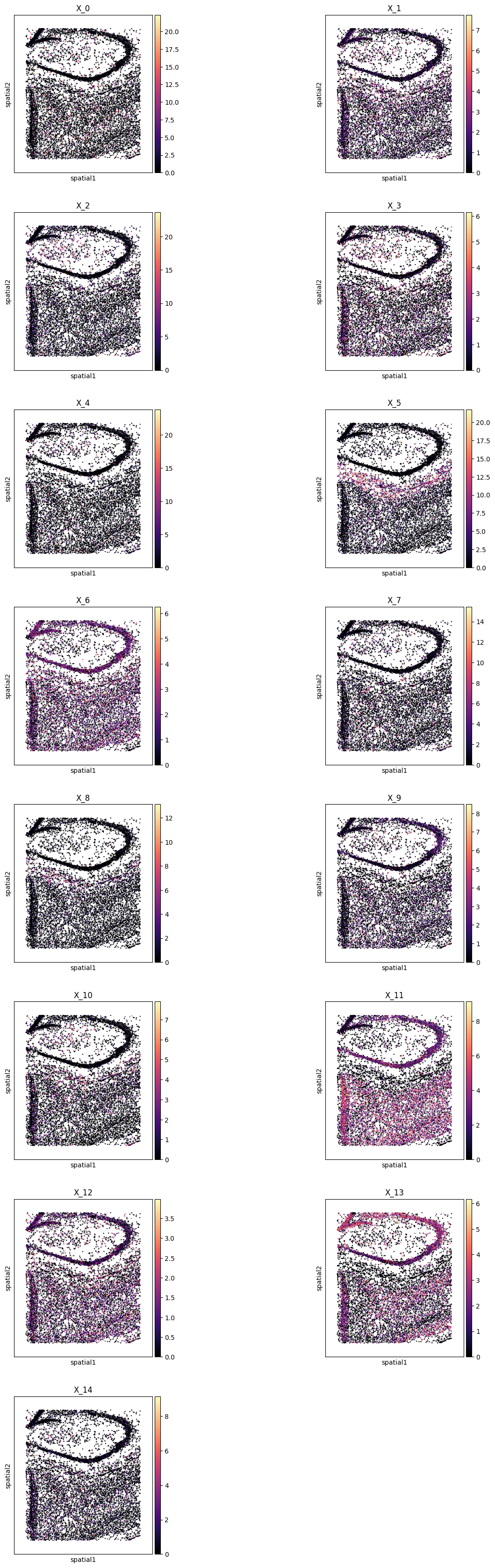
Plot all metagenes in-situ

pl.all_embeddings(demo, level=1, size=1, cmap="magma")

WARNING: Please specify a valid `library_id` or set it permanently in `adata.uns['spatial']`
WARNING: Please specify a valid `library_id` or set it permanently in `adata.uns['spatial']`

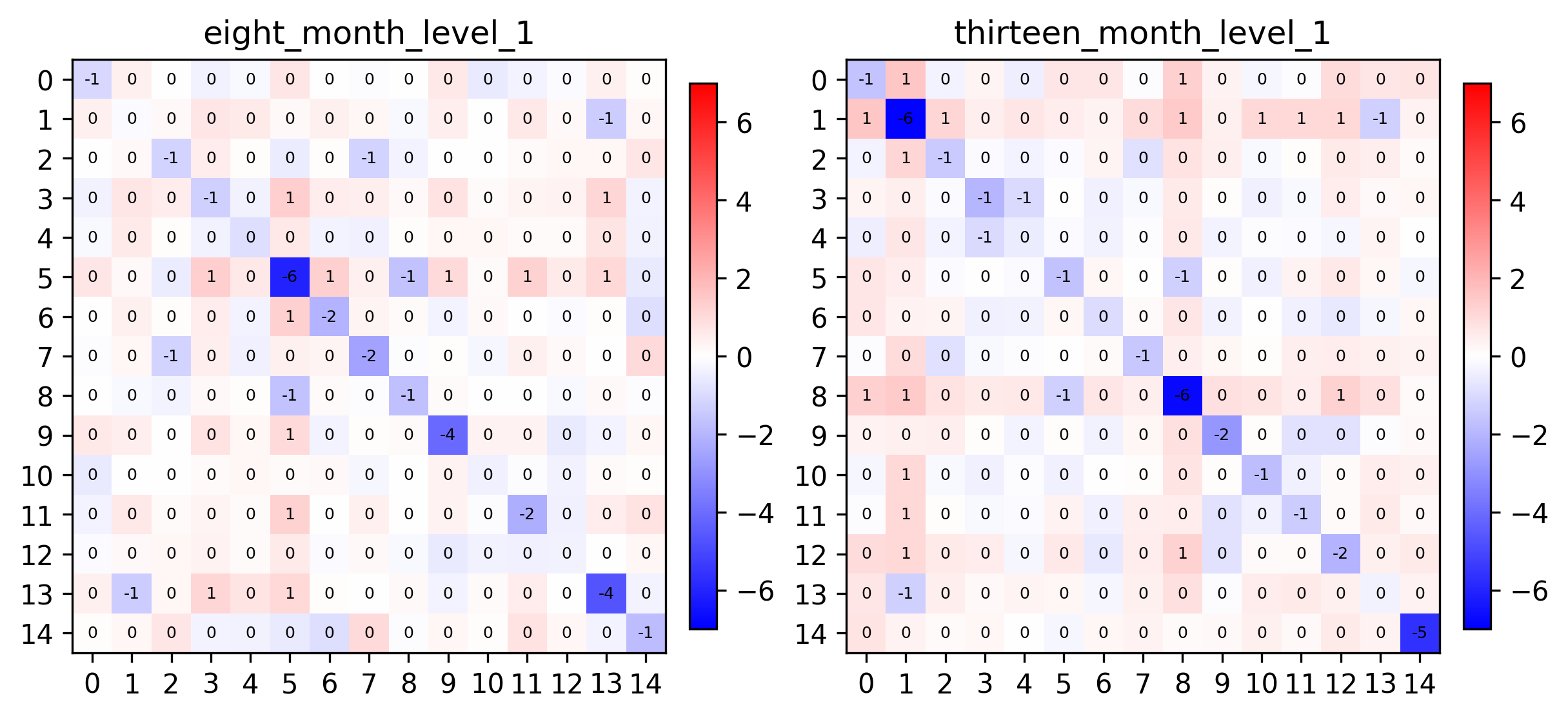
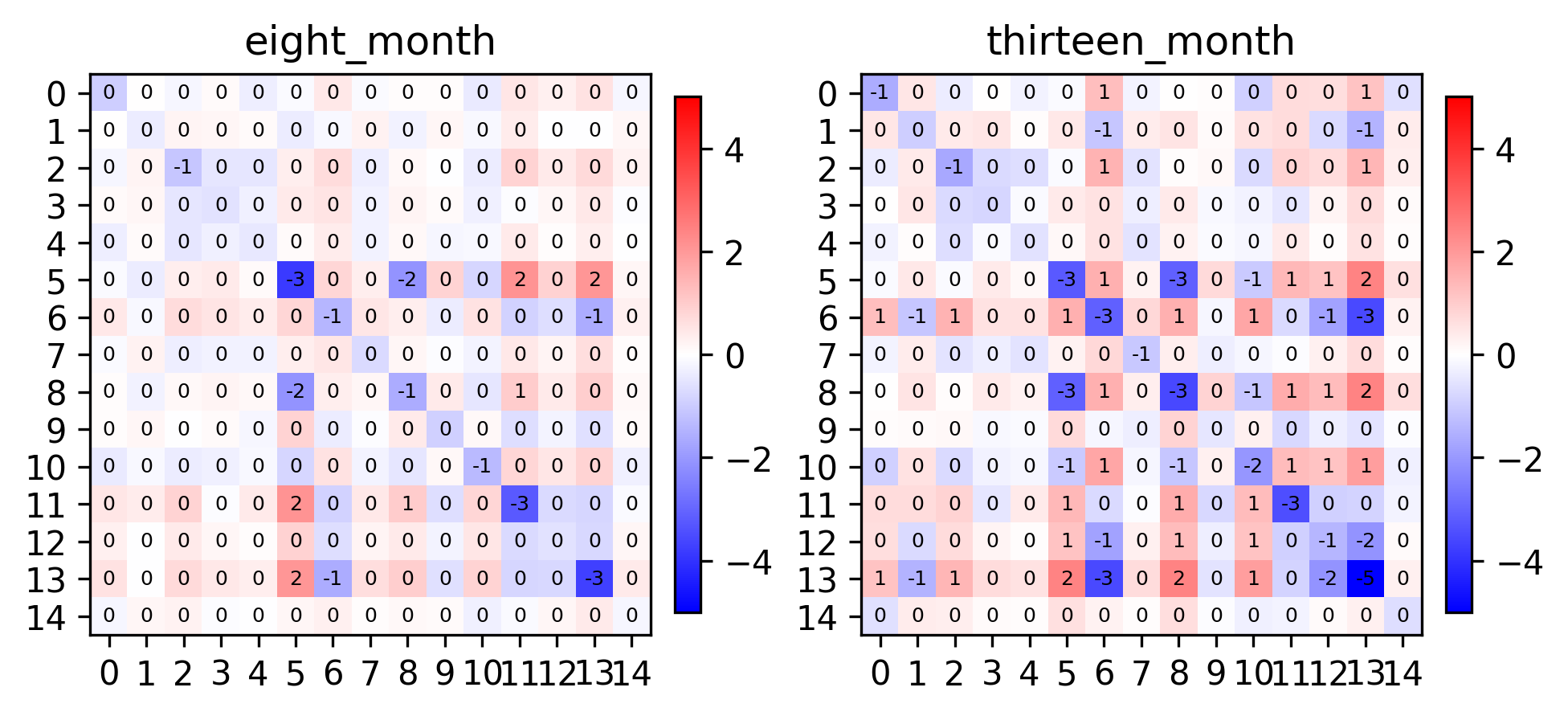
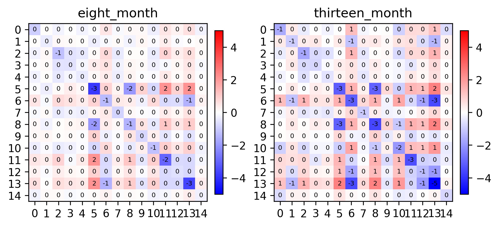
Comparing empirical correlations to learned affinities

fig, axes = plt.subplots(1, 2, figsize=(8, 8), constrained_layout=True, dpi=300)
pl.spatial_affinities(demo, level=1, label_values=True, label_font_size=6, axes=axes)

fig, axes = plt.subplots(1, 2, figsize=(8, 8), constrained_layout=True, dpi=300)
pl.spatial_affinities(demo, level=1, label_values=True, label_font_size=6, spatial_affinity_key="empirical_correlation", axes=axes)

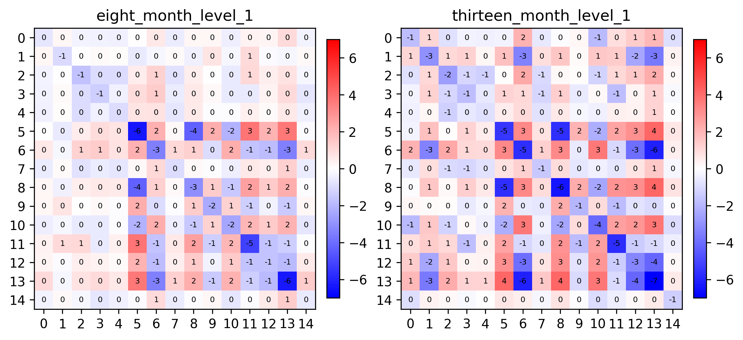
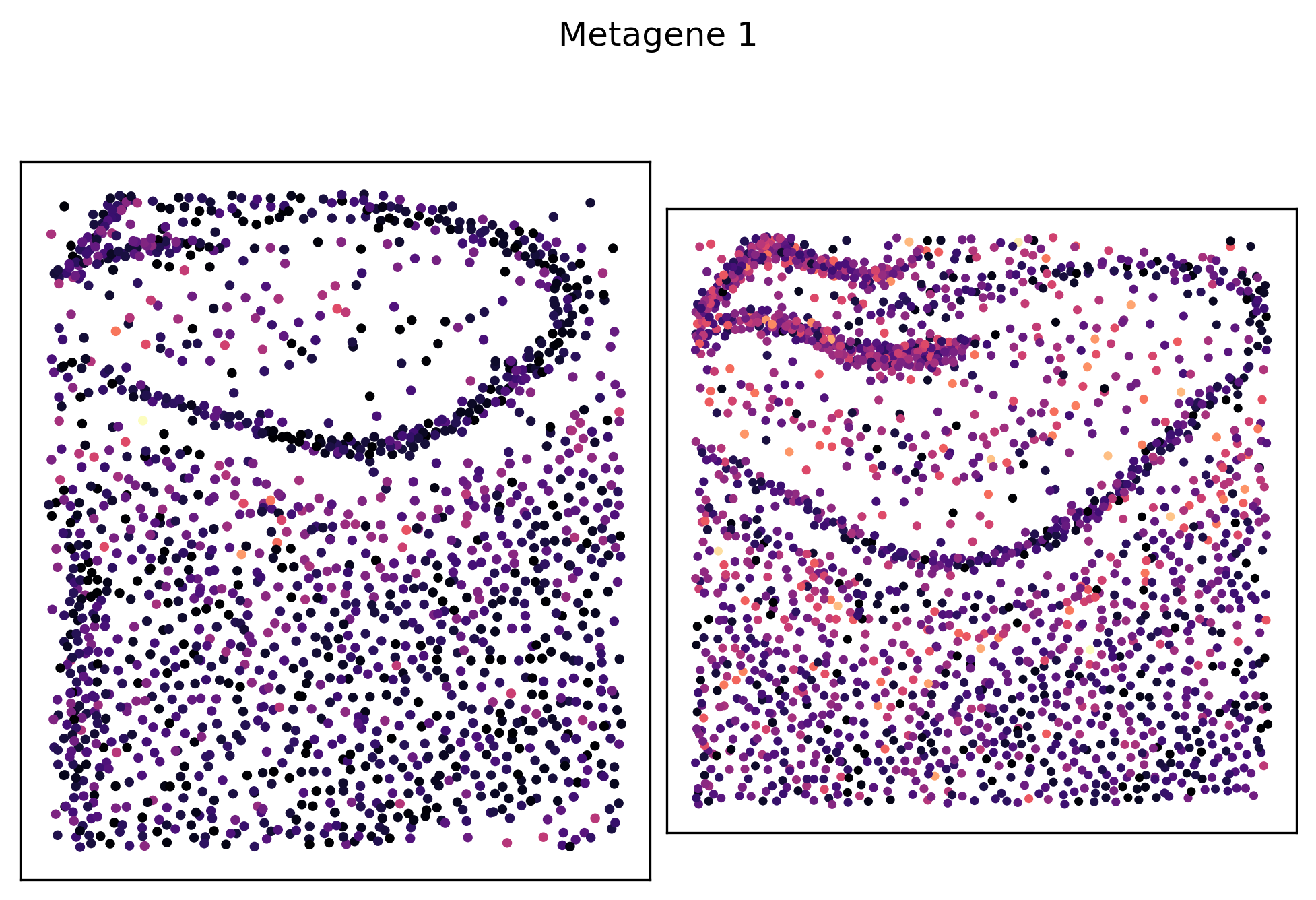
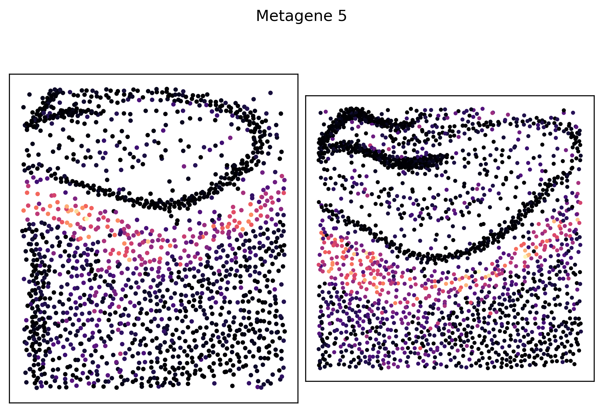
Plot particular metagenes

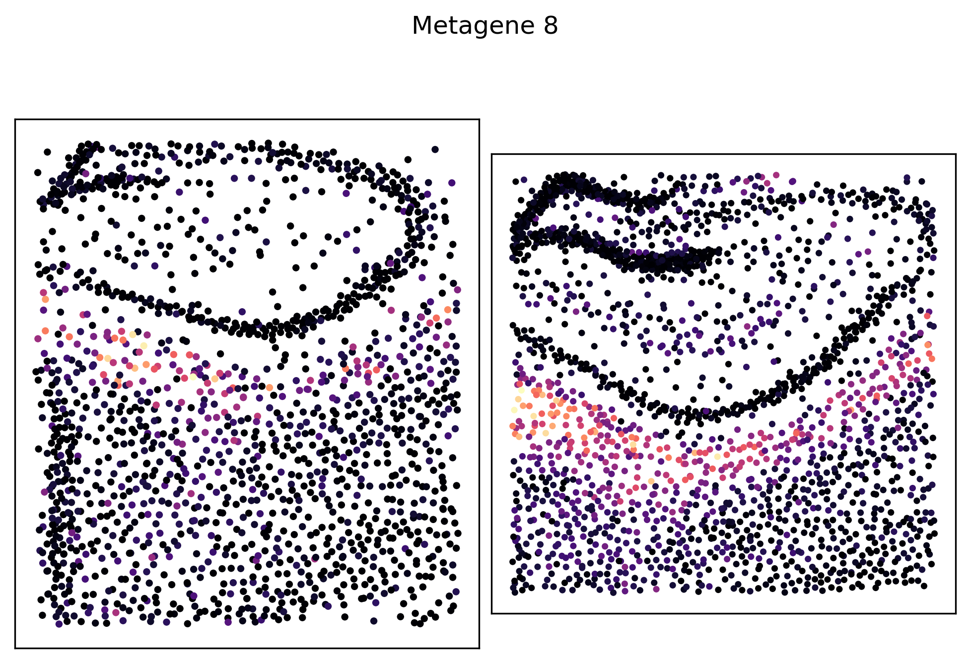
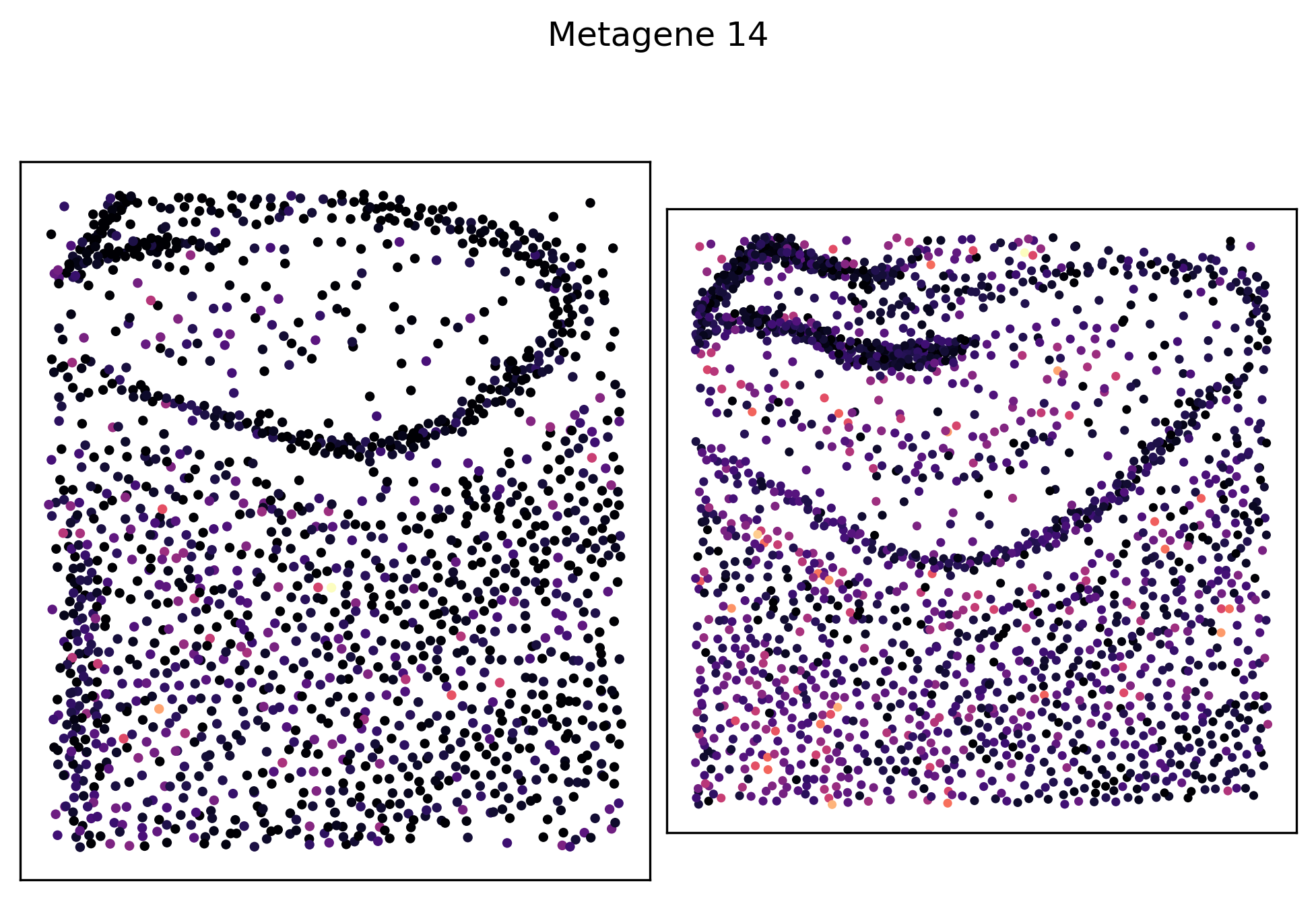
We can see that metagenes 1, 5, 8 and 14 have varying self-affinities between the two samples. Let’s visualize these metagenes in-situ distributions in particular:

_ = pl.metagene_embedding(demo, level=1, metagene_index=1, palette="magma")

_ = pl.metagene_embedding(demo, level=1, metagene_index=5, palette="magma")

_ = pl.metagene_embedding(demo, level=1, metagene_index=8, palette="magma")

_ = pl.metagene_embedding(demo, level=1, metagene_index=14, palette="magma")

# TODO: why do we need this step? It seems like the higher hierarhical levels don't have `var_names` copied correctly -> bug?
base_datasets = demo.hierarchy[0].datasets
for level in range(1, demo.hierarchical_levels):
    for dataset, base_dataset in zip(demo.hierarchy[level].datasets, base_datasets):
        dataset.var_names = base_dataset.var_names

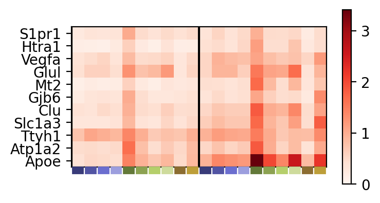
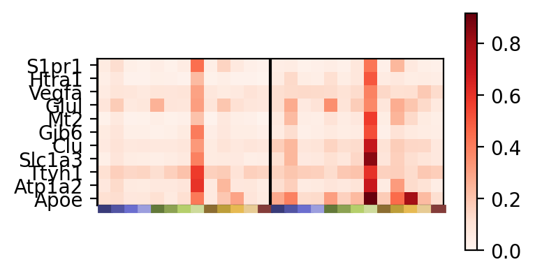
Plot differential metagene expression across domains

We can visualize the particular expression of top genes from a metagene and how these differ across the datasets and discovered spatial domains as a heatmap. Every n columns corresponds to the n discovered spatial domains for a particular dataset. The genes are in ranked order from most (bottom) to least (top) importance within the metagene.

_ = pl.metagene_signature_enrichment(demo, level=1, metagene_index=2, category_key="smoothed_domain", sensitivity=0.5)

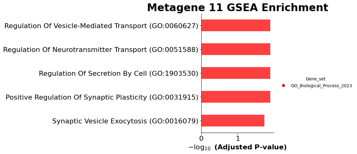
Metagene GO enrichment analysis

Using gseapy, we can evaluate the association of particular metagenes with GO terms. As shown below, Metagene 11 is associated with some important neuron signaling-related GO terms:

_ = tl.metagene_gsea(demo, sensitivity=0.5, metagene_index=11)

Note

All data (including input gene expression data, spatial coordinates, learned embeddings/metagenes/spatial affinities) can be found within the popari.model.Popari.datasets attribute. You can build your own analysis functions that access these data; see popari.analysis and popari._dataset_utils for examples.

Hierarchical analyses

Because we used the hierarchical setting, we can repeat our analyses at the original resolution of the data. This can be accomplished using the level parameter; level=0 indicates the highest (original) resolution, whereas level=model.hierarchical_levels - 1 indicates the lowest resolution.

demo.hierarchical_levels

2

Postprocessing

tl.preprocess_embeddings(demo, level=0, normalized_key="normalized_X")
tl.leiden(demo, joint=True, level=0, use_rep="normalized_X")
tl.compute_empirical_correlations(demo, level=0, feature="X")

Label propagation

tl.propagate_labels(demo, label_key="smoothed_domain")

Visualization

# Plot in-situ high resolution clusters
fig, axes = plt.subplots(1, 2, constrained_layout=True, dpi=300)
_ = pl.in_situ(demo, level=0, color="leiden", legend_fontsize="small", joint=True, connectivity_key=None, size=10, axes=axes, palette="tab20b")

# Plot propagated domain labels
fig, axes = plt.subplots(1, 2, constrained_layout=True, dpi=300)
_ = pl.in_situ(demo, level=0, color="smoothed_domain", legend_fontsize="small", joint=True, connectivity_key=None, size=10, axes=axes, palette="tab20b")

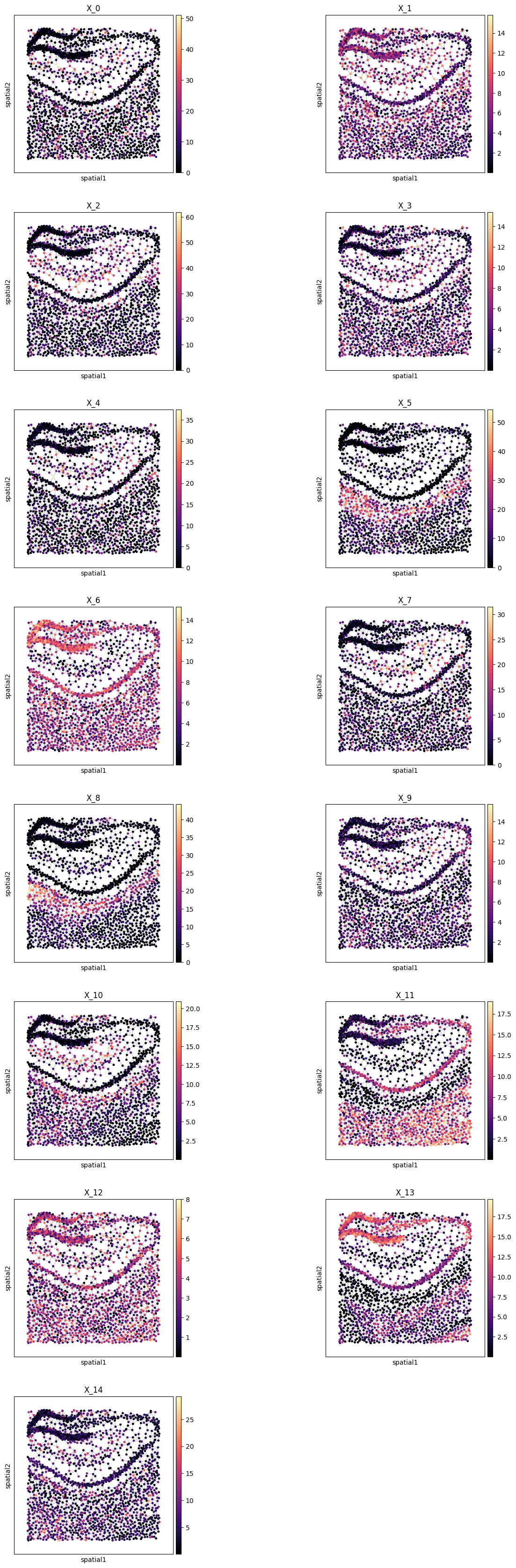
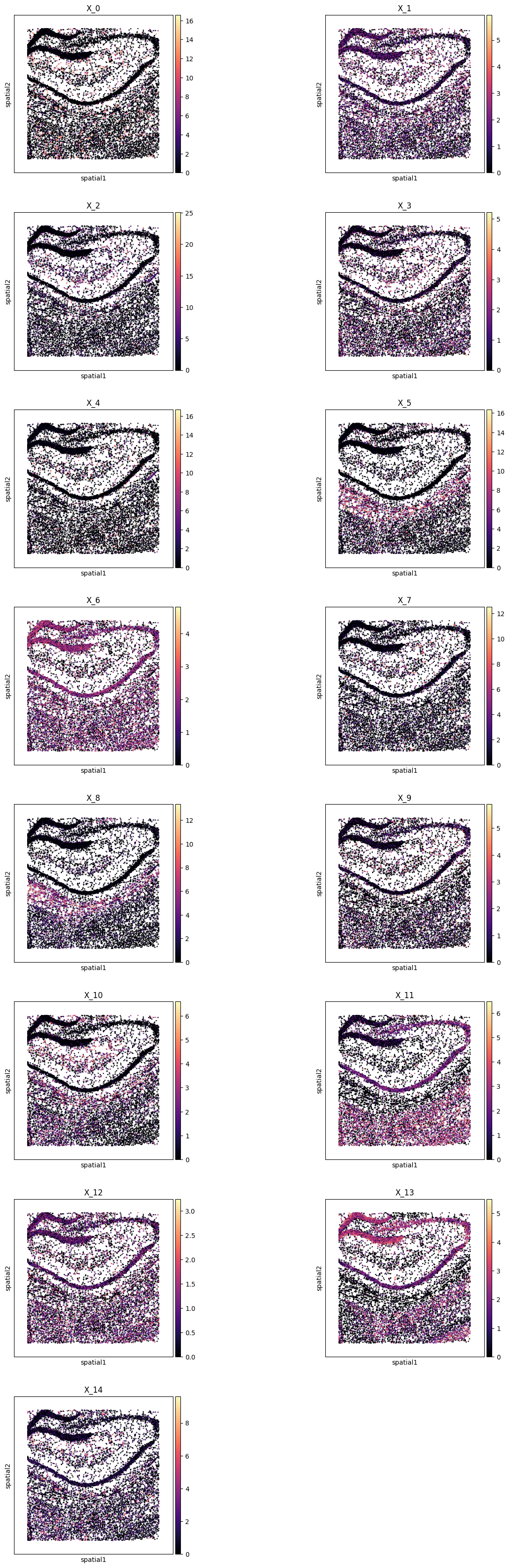
# Plot in-situ high resolution metagene embeddings
pl.all_embeddings(demo, level=0, size=0.1, edgecolors='none', cmap="magma")

WARNING: Please specify a valid `library_id` or set it permanently in `adata.uns['spatial']`
WARNING: Please specify a valid `library_id` or set it permanently in `adata.uns['spatial']`

fig, axes = plt.subplots(1, 2, constrained_layout=True, dpi=300)
pl.spatial_affinities(demo, level=0, label_values=True, label_font_size=6, axes=axes)

fig, axes = plt.subplots(1, 2, constrained_layout=True, dpi=300)
pl.spatial_affinities(demo, level=0, label_values=True, label_font_size=6, spatial_affinity_key="empirical_correlation", axes=axes)

_ = pl.metagene_signature_enrichment(demo, level=0, metagene_index=2, category_key="leiden", sensitivity=0.5)

_ = pl.metagene_signature_enrichment(demo, level=1, metagene_index=2, category_key="smoothed_domain", sensitivity=0.5)

Custom plotting function

You can create your own plotting functions using the popari._dataset_utils._broadcast_operator function.

# TODO